
Model One-Time Effects to Correct the Simulation Basis
How do you model One-Time effects that correct your simulation basis? This document will walk you through an example model and its formulas.
The Example Model
The example Model uses a Base Value, that is ideally obtained from your source system.
The revenue itself is then calculated as the forecasted revenue based on the corrected base value. Revenue from measures will be added as an assumption.
The formulas in detail:
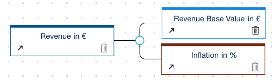
Revenue Base Value
EXPANDSINGLE(100,"Year","2018")
Simply use 100 as the base value. In real models, this usually uses the DATA function to get the latest actual data from an excel sheet or an external Data Source. The 100 is overwritten in a simulation by the corrected value.
Inflation
EXPAND(0,"Year")
The default value for inflation is usually 0. The actual inflation is added as an assumption later on.
Revenue
ROLLFORWARD('Revenue Base Value','Inflation')
The Rollforward function is used to create all future values of the Revenue. An assumption on this node will only influence the result, e.g. an additional line-item on revenue will be added as it is, with no additional inflation applied.
An Example in the Scenario Manager
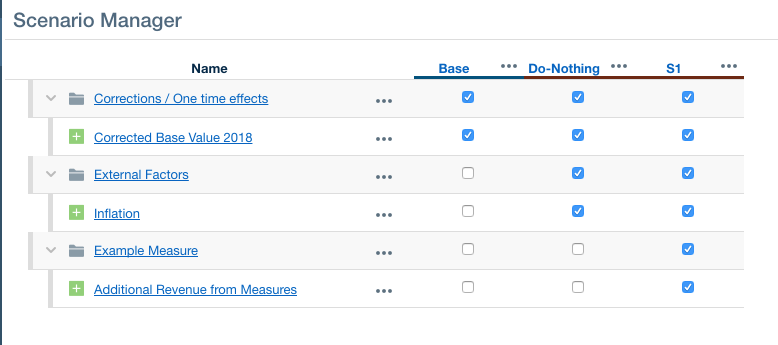
We create the “Base” & “Do-Nothing” scenario. The base correction only influences the base revenue and accounts for one-time effects that should not go into the basis for our simulation.
Inflation and other external factors that we cannot influence are assigned to the “Do-Nothing” scenario.
Finally, measures such as projects that we might start going into the first discussion scenario.
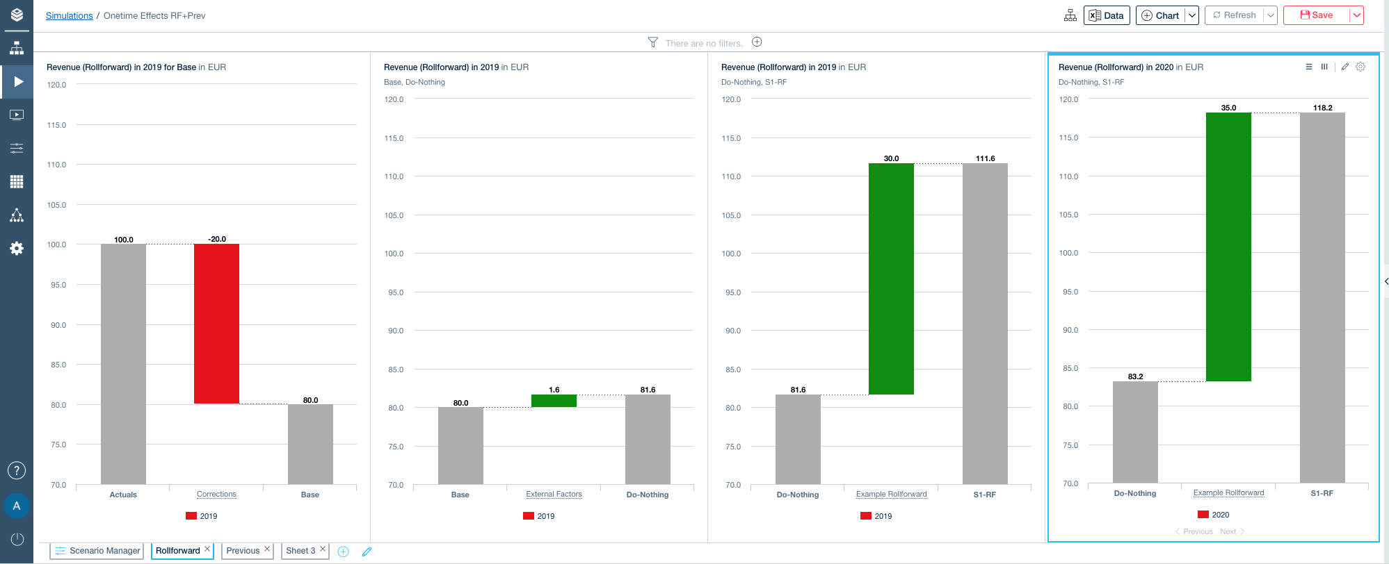
An exemplary Assumption Bridge
The following screenshot shows the example model with a base of 100, a correction of -20, an inflation of 2%, and an example measure of +30 in 2019, and +35 in 2020.
Advanced Modelling with a Previous Loop
Sometimes the rollforward function limitations are a show stopper, and you need the full-featured PREVIOUS function to model your problem. You can use similar techniques to create the corresponding Scenarios. We will extend the above Model with a previous loop to highlight the differences.
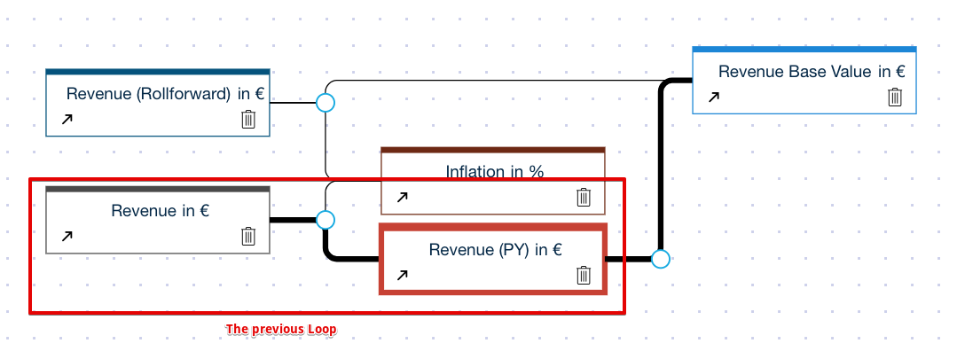
Revenue (PY)
PREVIOUS('Revenue', "Year" ,'Revenue Base Value', "2018")
Tells the Model to use the previous year's value of the revenue, except for 2018, where it uses the revenue base value.
Revenue
'Revenue (PY)'* ADDEACH('Inflation',1)
Revenue is calculated as the previous year's revenue times (Inflation+1). The addeach function essentially adds 1 to each value from the “Inflation” node.
Let's look at the differences in the simulation now. Since each value that we add as Assumption Line-Item on Revenue is now part of the loop, the values need to be entered as delta values to the previous year. Suppose we want to model a Line-Item that leads to 30 EUR extra revenue in 2019, 35 in 2020, and 40 in 2021. (all vs. the base year).
To enter this as an assumption line-item on revenue the following logic applies for the rollforward case and the previous case respectively:
Year | Assumption on Revenue node | Simulation Result on Revenue | ||
|---|---|---|---|---|
Rollforward | Previous | Rollforward | Previous | |
2018 | 0 | 0 | ||
2019 | +30 | +30 | 30 | 30 |
2020 | +35 | +5 | 35 | 35.6 (for inflation = 2%) |
2021 | +40 | +5 | 40 | 41.3 (w/ Inflation) |
As you can see, the main differences are the entry format of an assumption and if other factors are applied to the simulation values as well. You can read more at: